Slope Space in BRDF Theory
When you read BRDF theory papers, you’ll often see mention of slope space. Sometimes, components of the BRDF such as NDFs or masking-shadowing functions are defined in slope space, or operations are done in slope space before being converted back to ordinary vectors or polar coordinates. However, the meaning and intuition of slope space is rarely explained. Since it may not be obvious exactly what slope space is, why it is useful, or how to transform things to and from it, I thought I would write down a gentler introduction to it.
Slope Refresher
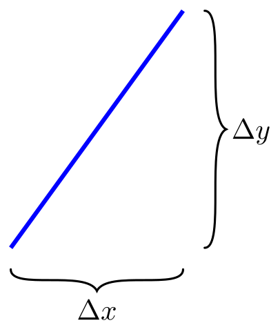
First off, what even is this “slope” thing we’re talking about? If you think back to your high school algebra class, the slope of a line was defined as “rise over run”, or the ratio $\Delta y / \Delta x$ between some two points on the line.

The steeper the line, the larger the magnitude of its slope. The sign of the slope indicates which direction the line is sloping in. The slope is infinite if the line is vertical.
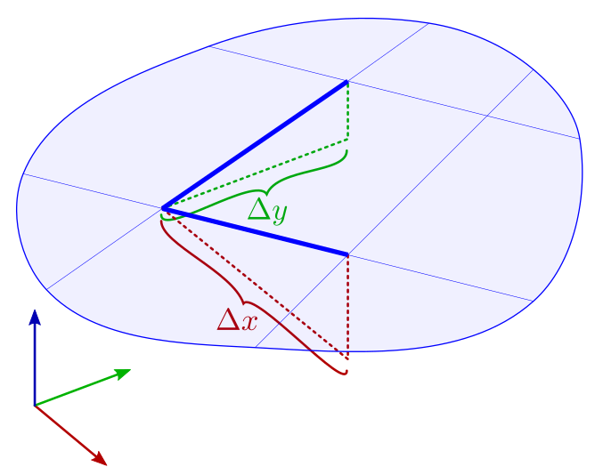
The concept of slope can readily be generalized to planes as well as lines. Planes have two slopes, one for $\Delta z / \Delta x$ and one for $\Delta z / \Delta y$ (using $z$-up coordinates, and assuming the surface is not vertical):

These values describe how much the surface rises or falls in $z$ if you take a step along either $x$ or $y$. This completely specifies the orientation of a planar surface, as steps in any other direction can be derived from the $x$ and $y$ slopes.
In calculus, the slope of a line is generalized to the derivative or “instantaneous slope” of a curve, $\mathrm{d}y/\mathrm{d}x$. For curved surfaces, so long as they can be expressed as a heightfield (where $z$ is a function of $x, y$), slopes become partial derivatives $\partial z / \partial x$ and $\partial z / \partial y$.
It’s worth noting that slopes are completely coordinate-dependent quantities. If you transform to a different coordinate system, the slopes of $z$ with respect to $x, y$ will be totally different values, or even infinite (if the surface is not a heightfield anymore in the new coordinates).
Normals and Slopes
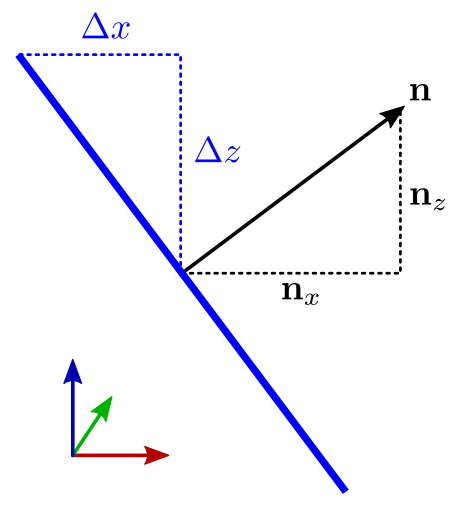
We usually describe surfaces in 3D by their normal vector rather than their slopes, as the normal is able to gracefully handle surfaces in any orientation without infinities, and is easier to transform into different coordinate systems. However, there is a simple relationship between a surface’s normal and its slopes, as this diagram should hopefully convince you:

The two triangles with the dotted lines in the figure are congruent (same angles and sizes), but rotated by 90 degrees. As the normal is, by definition, perpendicular to the surface, the normal’s components have the same proportionality as coordinate deltas along the surface, just swapped around. This diagram shows the $xz$ projection, but the same holds true of the $yz$ components: $$ \begin{aligned} \frac{\Delta z}{\Delta x} &= -\frac{\mathbf{n}_x}{\mathbf{n}_z} \\[1em] \frac{\Delta z}{\Delta y} &= -\frac{\mathbf{n}_y}{\mathbf{n}_z} \end{aligned} $$ The negative sign is because $\Delta z$ is going down while $\mathbf{n}_z$ is going up (or vice versa, depending on the orientation).
Just for completeness, when you have a heightfield surface $z(x, y)$, the partial derivatives are related to its normal at a point in the same way: $$ \begin{aligned} \frac{\partial z}{\partial x} &= -\frac{\mathbf{n}_x}{\mathbf{n}_z} \\[1em] \frac{\partial z}{\partial y} &= -\frac{\mathbf{n}_y}{\mathbf{n}_z} \end{aligned} $$
Slope Space
Now we’re finally ready to define slope space. Due to the relationship between slopes and normal vectors, slopes act as an alternate parameterization of unit vectors in the $z > 0$ hemisphere. Given any vector, we can treat it as a normal and find the slopes of a surface perpendicular to it. “Slope space” refers to this domain: the 2D space of all the possible slope values. As slopes can be any real numbers, slope space is just the real plane, $\mathbb{R}^2$, but with a special meaning.
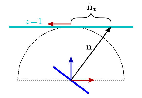
A good way to visualize slope space is to identify it with the plane $z = 1$. Then, vectors at the origin can be converted to slope space by intersecting them with the plane:

Here I’ve introduced the notation $\tilde{\mathbf{n}}$ for the 2D vector in slope space corresponding to the 3D vector $\mathbf{n}$. The tilde ($\sim$) notation for slope-space quantities is commonly used in the BRDF literature, and I’ll follow it here.
Intersecting a ray with the $z = 1$ plane is equivalent to rescaling the vector so that $\mathbf{n}_z = 1$, and then the slopes can be read off as the negated $x, y$ components of the rescaled vector. You can visualize the slope plane as having inverted $x, y$ axes compared to the base coordinates to take care of this. (Note the $x$-axis on the slope plane, pointing to the left, in the diagram above.)
So, you can picture the hemisphere being blown up and stretched onto the plane, by projecting each point away from the origin until it hits the plane. This establishes a bijection (one-to-one mapping) between the unit vectors with $z > 0$ and points on the plane.
To make it official, the slope-space parameterization of an arbitrary vector $\mathbf{v}$ with $\mathbf{v}_z > 0$ is defined by: $$ \begin{aligned} \tilde{\mathbf{v}}_x &= -\frac{\mathbf{v}_x}{\mathbf{v}_z} \\[1em] \tilde{\mathbf{v}}_y &= -\frac{\mathbf{v}_y}{\mathbf{v}_z} \end{aligned} $$ This assumes that the vector is upward-pointing, so that $\mathbf{v}_z > 0$. Finite slopes cannot represent horizontal vectors (normal to vertical surfaces), and they cannot distinguish between upward- and downward-pointing vectors, as slopes have no sense of orientation—reverse the normal, and you still get the same slopes.
Converting back from slopes to an ordinary unit normal vector is also simple: $$ \mathbf{v} = \text{normalize}(-\tilde{\mathbf{v}}_x, -\tilde{\mathbf{v}}_y, 1) $$
Converting to Polar Coordinates
Another common parameterization of unit vectors is the polar coordinates $\theta, \phi$. It’s straightforward to work out the direct conversion between slope space and polar coordinates.
Following common conventions, we define the polar coordinates so that $\theta$ measures downward from the $+z$ axis, and $\phi$ measures counterclockwise from the $+x$ axis. The conversion between polar and 3D unit vectors is: $$ \begin{aligned} \theta &= \text{acos}(z) \\ \phi &= \text{atan2}(y, x) \end{aligned} \qquad \begin{aligned} x &= \sin\theta \cos\phi \\ y &= \sin\theta \sin\phi \\ z &= \cos\theta \end{aligned} $$ and the conversion between polar and slope space is: $$ \begin{aligned} \theta &= \text{atan}(\sqrt{\tilde x^2 + \tilde y^2}) \\ \phi &= \text{atan2}(-\tilde y, -\tilde x) \end{aligned} \qquad \begin{aligned} \tilde x &= -\!\tan\theta \cos\phi \\ \tilde y &= -\!\tan\theta \sin\phi \\ \end{aligned} $$ This can be derived by setting $\tilde x = -x/z$ and substituting the conversion from polar, then using the identity $\sin/\cos = \tan$.
A fact worth noting here is that the magnitude of a slope-space vector, $|\tilde{\mathbf{v}}|$, is equal to $\tan\theta_\mathbf{v}$.
Properties of Slope Space
Now we’ve seen how to define slope space and convert back and forth from it. But why is it useful? Why would we want to represent vectors or functions in this way?
In microfacet BRDF theory, we usually assume the microsurface is a heightfield for simplicity (which is a pretty reasonable assumption for a lot of everyday materials). If the microsurface is a heightfield, then its normals are constrained to the upper hemisphere. Slope space, which parameterizes exactly the upper hemisphere, is a good match for this.
From a performance perspective, slope space is also much cheaper to transform to and from than polar coordinates, which makes it nicer to use in shaders. It requires only some divides or a normalize, as opposed to a bunch of forward or inverse trigonometric functions.
Slope space also has no boundaries, in contrast to other representations of unit vectors. The origin (0, 0) of the slope plane represents a flat surface normal, and the farther away you get, the more extreme the slope, but you can’t make the surface turn upside down or produce an invalid normal. So, you can freely do various manipulations on vectors in slope space without worrying about exceeding any bounds.
Another useful fact about slope space is that many linear transformations of a surface, such as scaling or shearing, map to transformations of its slope space in simple ways. For example, scaling a surface by a factor $\alpha$ along its $z$-axis causes its normal vectors’ $z$-components to scale by $1/\alpha$ (due to normals taking the inverse transpose), but then since $\mathbf{n}_z$ is in the denominator in the definition of slope space, we have that the slopes of the surface are scaled by $\alpha$.
Here’s a table of how transformations of the microsurface map to transformations of slope space:
| Surface | Slope Space |
|---|---|
| Horizontal scale by $(\alpha_x, \alpha_y)$ | Scale by $(1/\alpha_x, 1/\alpha_y)$ |
| Vertical scale by $\alpha$ | Scale by $\alpha$ |
| Horizontal rotate ($xy$) by $\theta$ | Rotate by $\theta$ |
| Vertical rotate ($xz, yz$) | Projective transform (not recommended) |
| Horizontal shear ($xy$) by $\begin{bmatrix} 1 & k_2 \\ k_1 & 1 \end{bmatrix}$ | Shear by $\begin{bmatrix} 1 & -k_1 \\ -k_2 & 1 \end{bmatrix}$ |
| Vertical shear by $\begin{bmatrix} 1 & 0 & 0 \\ 0 & 1 & 0 \\ k_x & k_y & 1 \end{bmatrix}$ | Translate by $(k_x, k_y)$ |
| Vertical shear by $\begin{bmatrix} 1 & 0 & k_x \\ 0 & 1 & k_y \\ 0 & 0 & 1 \end{bmatrix}$ | Projective transform (not recommended) |
These transformations in slope space are often exploited by parameterized BRDF models; they can implement roughness, anisotropy, and such as transformations applied to a single canonical BRDF (see for example Heitz 2014, section 5).
Distributions in Slope Space
One of the key ingredients in a microfacet BRDF is its normal distribution function (NDF), and one of the key uses for slope space is defining NDFs. Because slope space is an unbounded 2D plane, we can import existing 1D or 2D distribution functions and manipulate them in various ways, just as we would in any 2D domain. As long as we end up with a valid, normalized probability distribution in the slope plane (sometimes called a slope distribution function, or a $P^{22}$ function—I’m not sure where the latter term comes from), we can transform it to a properly normalized NDF expressed in polar or vector form. Let’s see how to do that.
The Jacobian
When mapping distribution functions from one space to another, it’s important to remember that the values of these functions are not dimensionless numbers; they are densities with respect to the area or volume measure of the underlying space. Therefore, it’s not enough just to change variables to express the function in the new coordinates; you also have to correct for the way the mapping stretches or squeezes the volume, which can vary from place to place.
Symbolically, suppose we have a domain $A$ with a probability density $p(a)$ defined on it. We want to map this to a domain $B$ parameterized by some new coordinates $b$. What we want is not just $p(a) = p(b)$ when $a \mapsto b$ under the mapping. Rather, we need to maintain: $$ p(a) \, \mathrm{d}A = p(b) \, \mathrm{d}B $$ where $\mathrm{d}A, \mathrm{d}B$ are matching volume elements of the respective spaces, with $\mathrm{d}A \mapsto \mathrm{d}B$ under the mapping we’re using. This says that the amount of probability (or whatever thing whose density we’re measuring) in the infinitesimal volume $\mathrm{d}A$ is conserved under the mapping; the same amount of probability is present in $\mathrm{d}B$.
This equation can be rewritten: $$ p(b) = p(a) \frac{\mathrm{d}A}{\mathrm{d}B} $$ The factor $\mathrm{d}A / \mathrm{d}B$ here is called the Jacobian, referring to the determinant of the Jacobian matrix which contains all the derivatives of the change of variables from $a$ to $b$. Actually, this is the inverse Jacobian, as the forward Jacobian for $A \to B$ would be $\mathrm{d}B / \mathrm{d}A$. The forward Jacobian is the factor by which the mapping stretches or squeezes volumes locally around a point. Because a probability density has volume in the denominator, it transforms using the inverse Jacobian.
So, when converting a slope-space distribution to an NDF, we have to multiply by the appropriate Jacobian. But how do we find out what that is? First off, we have to recall that NDFs are defined not as a density over solid angle in the hemisphere, but as a density over projected area on the $xy$ plane. Thus, it’s not enough to just find the Jacobian from slope space to polar coordinates; we also need to find the Jacobian from polar coordinates to projected area.
To do this, I find it easiest to use the formalism of differential forms. Explaining how those work is out of the scope of this article, but here’s an exposition I found useful. They’re essentially fields of dual $k$-vectors.
First, we can write down the $xy$ projected area element, $\mathrm{d}x \wedge \mathrm{d}y$, in terms of polar coordinates by differentiating the mapping from polar to Cartesian, which I’ll repeat here for convenience: $$ \begin{gathered} \left\{ \begin{aligned} x &= \sin\theta \cos\phi \\ y &= \sin\theta \sin\phi \\ z &= \cos\theta \end{aligned} \right. \\[2em] \begin{aligned} \mathrm{d}x \wedge \mathrm{d}y &= (\cos\theta\cos\phi\,\mathrm{d}\theta - \sin\theta\sin\phi\,\mathrm{d}\phi) \ \wedge \\ &\qquad (\cos\theta\sin\phi\,\mathrm{d}\theta + \sin\theta\cos\phi\,\mathrm{d}\phi) \\[0.5em] &= \cos\theta\sin\theta\cos^2\phi\,(\mathrm{d}\theta \wedge \mathrm{d}\phi) \ - \\ &\qquad \cos\theta\sin\theta\sin^2\phi\,(\mathrm{d}\phi \wedge \mathrm{d}\theta) \\[0.5em] &= \cos\theta\sin\theta\,(\mathrm{d}\theta \wedge \mathrm{d}\phi) \end{aligned} \end{gathered} $$ Then, we can do the same thing with the slope-space area element: $$ \begin{gathered} \left\{ \begin{aligned} \tilde x &= -\!\tan\theta \cos\phi \\ \tilde y &= -\!\tan\theta \sin\phi \\ \end{aligned} \right. \\[1.5em] \begin{aligned} \mathrm{d}\tilde x \wedge \mathrm{d} \tilde y &= -(\cos^{-2}\theta\cos\phi\,\mathrm{d}\theta - \tan\theta\sin\phi\,\mathrm{d}\phi) \ \wedge \\ &\qquad -(\cos^{-2}\theta\sin\phi\,\mathrm{d}\theta + \tan\theta\cos\phi\,\mathrm{d}\phi) \\[0.5em] &= \tan\theta\cos^{-2}\theta\cos^2\phi\,(\mathrm{d}\theta \wedge \mathrm{d}\phi) \ - \\ &\qquad \tan\theta\cos^{-2}\theta\sin^2\phi\,(\mathrm{d}\phi \wedge \mathrm{d}\theta) \\[0.5em] &= \frac{\tan\theta}{\cos^2\theta} \, (\mathrm{d}\theta \wedge \mathrm{d}\phi) \end{aligned} \end{gathered} $$ Now, all we have to do is divide: $$ \begin{aligned} \frac{\mathrm{d}\tilde x \wedge \mathrm{d} \tilde y}{\mathrm{d}x \wedge \mathrm{d}y} &= \frac{\tan\theta}{\cos^2\theta} \frac{1}{\cos\theta\sin\theta} \\[1em] &= \frac{1}{\cos^4\theta} \end{aligned} $$ Et voilà! The Jacobian for converting densities from slope space to NDF form is $1/\cos^4\theta$. We’ll have to multiply by this factor in addition to changing variables.
Some Common Distributions
As an example of the conversion from slope space to NDF, let’s take the standard (bivariate) Gaussian distribution defined on slope space: $$ D(\tilde{\mathbf{m}}, \sigma) = \frac{1}{2\pi\sigma^2} \exp\left(-\frac{|\tilde{\mathbf{m}}|^2}{2\sigma^2}\right) $$ To turn this into an NDF, we need to change variables from $\tilde{\mathbf{m}}$ to $(\theta_\mathbf{m}, \phi_\mathbf{m})$, and also multiply by the Jacobian $1/\cos^4\theta_\mathbf{m}$. Recalling that $|\tilde{\mathbf{m}}| = \tan\theta_\mathbf{m}$, this becomes: $$ D(\mathbf{m}, \sigma) = \frac{1}{2\pi\sigma^2\cos^4\theta_\mathbf{m}} \exp\left(-\frac{\tan^2\theta_\mathbf{m}}{2\sigma^2}\right) $$ Hey, that looks familiar—it’s the Beckmann NDF! (Although it’s more usually seen with the roughness parameter $\alpha = \sqrt{2}\sigma$.) The Beckmann distribution is a Gaussian in slope space.
The isotropic GGX NDF (Walter et al 2007) looks like this: $$ D(\mathbf{m}, \alpha) = \frac{\alpha^2}{\pi \cos^4\theta_\mathbf{m} \bigl(\alpha^2 + \tan^2\theta_\mathbf{m} \bigr)^2 } $$ You might now recognize those familiar-looking $\cos^4\theta_\mathbf{m}$ and $\tan\theta_\mathbf{m}$ factors. Yep, this NDF is also a convert from slope space! Working backwards, we can see that it was originally: $$ D(\tilde{\mathbf{m}}, \alpha) = \frac{\alpha^2}{\pi \bigl(\alpha^2 + |\tilde{\mathbf{m}}|^2 \bigr)^2 } $$ Although this formula is probably less familiar, it matches the pdf of the bivariate Student’s $t$-distribution with the “normality” parameter $\nu$ set to 2, and scaled by $\alpha/\sqrt{2}$. (You can also create a family of NDFs that interpolate between GGX and Beckmann, by exposing a user parameter that controls $\nu$; see Ribardière et al 2017.)
(Incidentally, the GGX NDF is often seen written in this alternate form: $$ D(\mathbf{m}, \alpha) = \frac{\alpha^2}{\pi \bigl( (\alpha^2 - 1)\cos^2\theta_\mathbf{m} + 1 \bigr)^2 } $$ This is the same function as the form above (which is from the original GGX paper), but rearranged to make it cheaper to evaluate, as it eliminates the $\tan^2$ using the identity $\tan^2 = (1 - \cos^2)/\cos^2$. However, this form also introduces numerical precision problems, and Filament has a numerically stable form: $$ D(\mathbf{m}, \alpha) = \frac{\alpha^2}{\pi \bigl(\alpha^2 \cos^2\theta_\mathbf{m} + \sin^2\theta_\mathbf{m} \bigr)^2 } $$ which is again the same function, rearranged some more; you’re meant to calculate $\sin^2\theta_\mathbf{m}$ as the squared magnitude of the cross product $|\mathbf{n} \times \mathbf{m}|^2$. This has nothing to do with slope space; I just thought it was neat and worth knowing.)
Conclusion
To recap, the most important thing to take away about slope space is that it provides an alternate representation for unit vectors in the upper hemisphere, by projecting them out onto an infinite plane. This enables us to work with distributions in plain old 2D space, and then map them back into functions on the hemisphere. Slope space also provides convenient mappings from some linear transformations of the microsurface to linear or affine transformations in the slope plane.
I hope this has demystified the concept of slope space a little bit, and now you won’t be confused by it anymore when reading BRDF papers! 😄